基于多策略自适应差分正余弦算法的多机器人路径规划Multi-robot path planning

1、简介

最近进行了使用各种元启发式算法进行多机器人路径规划的研究。其中一种算法正弦余弦算法（SCA）不能在路径规划问题中产生令人满意的结果，由于单一的更新策略。有必要采用多种更新策略，并针对更广泛的问题提高其性能。我们提出了一种新的多策略自适应微分正弦余弦算法（sdSCA），它使用策略池，并允许更频繁地选择策略，从而导致更好的解决方案，将sdSCA应用于具有静态和动态障碍物的复杂环境中的在线多机器人路径规划。

2、基本正弦余弦算法(SCA)

SCA是Mirjalili于2016年提出的基于数学的先进元启发式算法。该算法在更新解时采用正弦和余弦函数构建的方程，这些三角函数能有效利用两个不同解之间的空间(Mirjalili, 2016)。算法流程如下：首先通过式(1)随机生成初始种群：

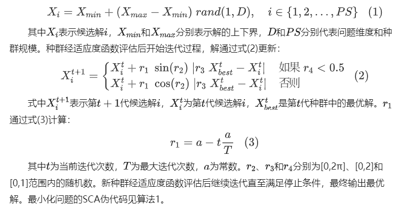
其中t为当前迭代次数，T为最大迭代次数，a为常数。r2、r3和r4分别为[0,2π]、[0,2]和[0,1]范围内的随机数。新种群经适应度函数评估后继续迭代直至满足停止条件，最终输出最优解。最小化问题的SCA伪代码见算法1。

3、多策略自适应差分正弦余弦算法(sdSCA)

基于种群的元启发式算法首先生成随机初始种群，经适应度函数评估后开始迭代更新过程。多数算法中，种群候选解通常采用单一更新策略，迭代结束时输出最优解。然而单一更新策略会限制算法搜索性能。SCA作为基于种群的算法，其原始更新策略如式(2)所示。

为突破这一限制，本文在SCA原有策略基础上引入差分策略，提出新型多策略自适应差分正弦余弦算法(sdSCA)。该算法中，每个候选解通过轮盘赌概率计算自主选择更新策略（非随机选择），算法自适应学习产生更优结果的策略，从而提升基础SCA的搜索性能。所提算法在基础SCA更新方程外新增三种差分策略，分别如式(4)、式(5)和式(6)所示：

算法流程说明：首先由式(2)、(4)-(6)构建包含四种差分策略的策略池，初始阶段各策略选择概率均设为25%。通过式(1)随机生成初始种群后，各候选解采用轮盘赌技术选择策略。经适应度函数评估后开始迭代，候选解按各自策略更新，同时更新策略选择计数器。新种群评估后，按式(7)计算各策略更新概率：

4、多机器人在线路径规划建模

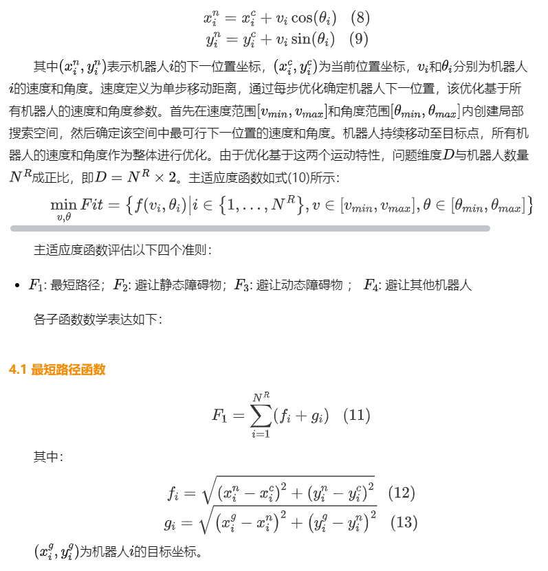
多机器人在线路径规划是一个最小化问题，旨在使机器人在复杂环境中逐步到达目标点，同时以最小成本避免与静态/动态障碍物及其他机器人碰撞(Toufan & Nitzade, 2020)。本文针对圆形同构多机器人系统进行在线路径规划仿真，机器人下一位置可通过式(8)-(9)计算：

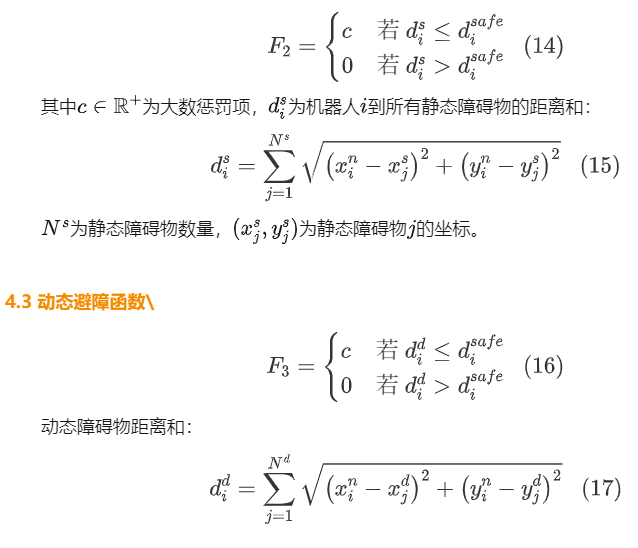
4.2 静态避障函数

5、算法性能评估指标

本文通过步数、移动距离、路径偏差误差、未达目标距离、总适应度和执行时间等指标评估算法性能。下面对路径偏差误差和未达目标距离进行详细说明。

5.1 平均路径偏差误差(APDE)

在迭代开始前，路径规划算法会为每个机器人计算数学上的理想路径（起点到目标的直线）。路径偏差误差(PDE)指算法实际路径与理想路径的距离差，第次运行的PDE计算如式(23)：

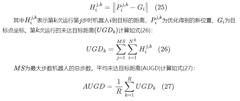
5.2 平均未达目标距离(AUGD)

当步数最多的机器人到达目标点时算法终止运行。在此过程中记录每个机器人每步到目标点的距离，欧氏距离计算如式(25)：

6、多机器人路径规划求解算法

提出的算法被应用于多机器人在线路径规划。仿真中机器人均为圆形、同构且尺寸统一，动态障碍物以恒定速度在两特定点间线性移动。研究构建了三个包含静态和动态障碍物的场景（单位：厘米）：

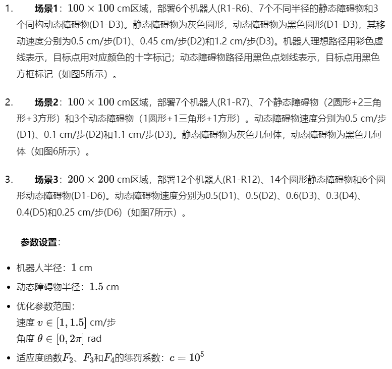
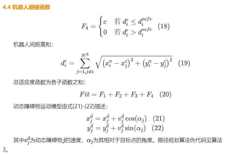
动态障碍物的速度设计旨在限制机器人运动并增加问题复杂度。各场景中机器人理想路径用彩色虚线表示，目标点用同色十字标记；动态障碍物路径用黑色点划线表示，目标点用黑色方框标记。

图1 场景1

% data of scenario 1
% ===================================================================
totalRobot =?6;?% number of robot
robotRadius =?ones(1, totalRobot);?% radius of robot
robotStart.x = [52545958595];?% start positions (x) of robots
robotStart.y = [95107595405];?% start positions (y) of robots
robotGoal.x = ?[402510654065];?% goal positions (x) of robots
robotGoal.y = ?[139755154075];?% goal positions (y) of robots
totalStatic =?7;?% number of static obstacles
staticRadius = [4335453];?% radius of static obstacles
static.x = [10252540357585];?% positions (x) of static obstacles
static.y = [80903065254015];?% positions (y) of static obstacles
totalDynamic =?3; ?% number of dynamic obstacles
dynamicRadius =?1.5?*?ones(1, totalDynamic);?% radius of dynamic obstacles
dynamicStart.x = [155575];?% start positions (x) of dynamic obstacles
dynamicStart.y = [402090];?% start positions (y) of dynamic obstacles
dynamicGoal.x = [355095];?% goal positions (x) of dynamic obstacles
dynamicGoal.y = [855075];?% goal positions (y) of dynamic obstacles
dynamicVelocity = [0.50.451.2];?% velocities of dynamic obstacles
axisParameter =?100;?% visualization scale (100 x 100)
% ===================================================================
% initial visualization
% ===================================================================
figure
alpha =?linspace(0,?2*pi,?100);
set(gcf,?'Position', [500,?20,?950,?950]);
ax = gca;
ax.Units =?'normalized';?
ax.Position = [0.0500.91];?
plt1 =?plot(-7,-7,'o','MarkerFaceColor',[0.50.50.5],'MarkerEdgeColor','k','MarkerSize',12);
hold?on;
plt2 =?plot(-8,-8,'o','MarkerFaceColor',[0.50.70.8],'MarkerEdgeColor','k','MarkerSize',12);
plt3 =?plot(-9,-9,'o','MarkerFaceColor',[0.10.20.9],'MarkerEdgeColor','k','MarkerSize',12);
fori?=?1?: totalStatic
? ??ifi?==?2?||?i?==?4
? ? ? ? x_square = [static.x(i) - staticRadius(i), static.x(i) + staticRadius(i), static.x(i) + staticRadius(i), static.x(i) - staticRadius(i)];
? ? ? ? y_square = [static.y(i) - staticRadius(i), static.y(i) - staticRadius(i), static.y(i) + staticRadius(i), static.y(i) + staticRadius(i)];
? ? ? ? plt10 = fill(x_square, y_square, [0.50.50.5]);
? ??elseifi?==?3?||?i?==?5
? ? ? ? x_tri = [static.x(i), static.x(i) - staticRadius(i) *?sqrt(3) /?2, static.x(i) + staticRadius(i) *?sqrt(3) /?2, static.x(i)];
? ? ? ? y_tri = [static.y(i) + staticRadius(i), static.y(i) - staticRadius(i) /?2, static.y(i) - staticRadius(i) /?2, static.y(i) + staticRadius(i)];
? ? ? ? plt10 = fill(x_tri, y_tri, [0.50.50.5]);
? ??else
? ? ? ? plt10 = fill(static.x(i) + staticRadius(i) *?cos(alpha), static.y(i) + staticRadius(i) *?sin(alpha), [0.50.50.5]);
? ??end
end
fori?=?1?: totalRobot
? ? plt11(i) = fill(robotStart.x(i) + robotRadius(i) *?cos(alpha), robotStart.y(i) + robotRadius(i) *?sin(alpha), [0.50.70.8]);
? ? plt4 =?plot(robotGoal.x(i), robotGoal.y(i),'x','MarkerFaceColor','k','MarkerEdgeColor','k','MarkerSize',10,'LineWidth',2);
? ? plt5 = line([robotStart.x(i) robotGoal.x(i)], [robotStart.y(i) robotGoal.y(i)],'Color','black','LineStyle','--');
end
fori?=?1?: totalDynamic
? ? plt12(i) = fill(dynamicStart.x(i) + dynamicRadius(i) *?cos(alpha), dynamicStart.y(i) + dynamicRadius(i) *?sin(alpha), [0.10.20.9]);
? ? plt6 =?plot(dynamicGoal.x(i), dynamicGoal.y(i),'x','MarkerFaceColor','b','MarkerEdgeColor','b','MarkerSize',10,'LineWidth',2);
? ? plt7 = line([dynamicStart.x(i) dynamicGoal.x(i)], [dynamicStart.y(i) dynamicGoal.y(i)],'Color','blue','LineStyle','--');
end
legend([plt2 plt1 plt3], {'(6) Robots','(7) Static obstacles',?'(3) Dynamic obstacles'},'FontSize',14,'Location','north');
axis equal;
axis([-5?(axisParameter+5)?0?(axisParameter)]);
pause(1);
% ===================================================================
saveas(gcf,'scenarioscenario1.emf'); ??

图2 场景2

% data of scenario 2
% ===================================================================
totalRobot =?12;?% number of robot
robotRadius =?ones(1, totalRobot);?% radius of robot
robotStart.x = [8? ??13? ??29? ??34? ??39? ??50? ??60? ??60? ??60? ??66? ??97? ??97];?% start positions (x) of robots
robotStart.y = [31? ??11? ??78? ??31? ??89? ??63? ??31? ??84? ??94? ??63? ??42? ??86];?% start positions (y) of robots
robotGoal.x = ?[18? ??13? ??29? ??18? ??39? ??76? ?102? ??81? ??87? ??34? ??97? ??97];?% goal positions (x) of robots
robotGoal.y = ?[47? ??90? ??16? ??31? ??47? ??26? ??58? ??94? ??73? ? ?5? ??79? ??94];?% goal positions (y) of robots
totalStatic =?9;?% number of static obstacles
staticRadius = [221322324];?% radius of static obstacles
static.x = [132534292958856813];?% positions (x) of static obstacles
static.y = [403131456550478870];?% positions (y) of static obstacles
totalDynamic =?5; ?% number of dynamic obstacles
dynamicRadius =?1.5?*?ones(1, totalDynamic);?% radius of dynamic obstacles
dynamicStart.x = [40? ??24? ??3466? ??92]; ?% start positions (x) of dynamic obstacles
dynamicStart.y = [40? ??47? ??8426? ??63];?% start positions (y) of dynamic obstacles
dynamicGoal.x = [60? ??34? ??4576? ?100];?% goal positions (x) of dynamic obstacles
dynamicGoal.y = [15? ??68? ??6352? ??65];?% goal positions (y) of dynamic obstacles
dynamicVelocity =?rand(1,totalDynamic) +?0.2;?% velocities of dynamic obstacles
axisParameter =?100;?% visualization scale (100 x 100)
% ===================================================================
% initial visualization
% ===================================================================
figure
alpha =?linspace(0,?2*pi,?100);
set(gcf,?'Position', [500,?20,?950,?950]);
ax = gca;
ax.Units =?'normalized';?
ax.Position = [0.0500.91];?
plt1 =?plot(-7,-7,'o','MarkerFaceColor',[0.50.50.5],'MarkerEdgeColor','k','MarkerSize',12);
hold?on;
plt2 =?plot(-8,-8,'o','MarkerFaceColor',[0.50.70.8],'MarkerEdgeColor','k','MarkerSize',12);
plt3 =?plot(-9,-9,'o','MarkerFaceColor',[0.10.20.9],'MarkerEdgeColor','k','MarkerSize',12);
fori?=?1?: totalStatic
? ??ifi?==?2?||?i?==?5?||?i?==?7
? ? ? ? x_square = [static.x(i) - staticRadius(i), static.x(i) + staticRadius(i), static.x(i) + staticRadius(i), static.x(i) - staticRadius(i)];
? ? ? ? y_square = [static.y(i) - staticRadius(i), static.y(i) - staticRadius(i), static.y(i) + staticRadius(i), static.y(i) + staticRadius(i)];
? ? ? ? plt10 = fill(x_square, y_square, [0.50.50.5]);
? ??elseifi?==?3?||?i?==?5?||?i?==?8
? ? ? ? x_tri = [static.x(i), static.x(i) - staticRadius(i) *?sqrt(3) /?2, static.x(i) + staticRadius(i) *?sqrt(3) /?2, static.x(i)];
? ? ? ? y_tri = [static.y(i) + staticRadius(i), static.y(i) - staticRadius(i) /?2, static.y(i) - staticRadius(i) /?2, static.y(i) + staticRadius(i)];
? ? ? ? plt10 = fill(x_tri, y_tri, [0.50.50.5]);
? ??else
? ? ? ? plt10 = fill(static.x(i) + staticRadius(i) *?cos(alpha), static.y(i) + staticRadius(i) *?sin(alpha), [0.50.50.5]);
? ??end
end
fori?=?1?: totalRobot
? ? plt11(i) = fill(robotStart.x(i) + robotRadius(i) *?cos(alpha), robotStart.y(i) + robotRadius(i) *?sin(alpha), [0.50.70.8]);
? ? plt4 =?plot(robotGoal.x(i), robotGoal.y(i),'x','MarkerFaceColor','k','MarkerEdgeColor','k','MarkerSize',10,'LineWidth',2);
? ? plt5 = line([robotStart.x(i) robotGoal.x(i)], [robotStart.y(i) robotGoal.y(i)],'Color','black','LineStyle','--');
end
fori?=?1?: totalDynamic
? ? plt12(i) = fill(dynamicStart.x(i) + dynamicRadius(i) *?cos(alpha), dynamicStart.y(i) + dynamicRadius(i) *?sin(alpha), [0.10.20.9]);
? ? plt6 =?plot(dynamicGoal.x(i), dynamicGoal.y(i),'x','MarkerFaceColor','b','MarkerEdgeColor','b','MarkerSize',10,'LineWidth',2);
? ? plt7 = line([dynamicStart.x(i) dynamicGoal.x(i)], [dynamicStart.y(i) dynamicGoal.y(i)],'Color','blue','LineStyle','--');
end
legend([plt2 plt1 plt3], {'(12) Robots',?'(9) Static obstacles',?'(5) Dynamic obstacles'},'FontSize',14,'Location','southeast');
axis equal;
axis([-5?(axisParameter+5)?0?(axisParameter)]);
pause(1);
% ===================================================================
saveas(gcf,'scenarioscenario2.emf'); ? ??

图3 场景3

% data of scenario 3
% ===================================================================
totalRobot =?20;?% number of robot
robotRadius =?ones(1, totalRobot);?% radius of robot
robotStart.x = [5525251085406045726010514514514510010050100120] ;?% start positions (x) of robots
robotStart.y = [1351005100585408045726013014511080201251510025];?% start positions (y) of robots
robotGoal.x = ?[25255751540708051209012014514514512512575130140];?% goal positions (x) of robots
robotGoal.y = ?[135125251258512514080707230110120903060125158025];?% goal positions (y) of robots
totalStatic =?13;?% number of static obstacles
staticRadius = [5354333344553];?% radius of static obstacles
static.x = [1210043553011050145145145145115107];?% positions (x) of static obstacles
static.y = [45726090551207050651001309032];?% positions (y) of static obstacles
totalDynamic = ?7; ?% number of dynamic obstacles
dynamicRadius =?1.5?*?ones(1, totalDynamic);?% radius of dynamic obstacles
dynamicStart.x = [155030601710075]; ?% start positions (x) of dynamic obstacles
dynamicStart.y = [145140803056055] ;?% start positions (y) of dynamic obstacles
dynamicGoal.x = [157060632513560];?% goal positions (x) of dynamic obstacles
dynamicGoal.y = [10070755154040];?% goal positions (y) of dynamic obstacles
dynamicVelocity =?rand(1,totalDynamic) +?0.2;?% velocities of dynamic obstacles
axisParameter =?150;?% visualization scale (150 x 150)
% ===================================================================
% Robots path's colors
% ===================================================================
Colors = jet(totalRobot);
% Colors = (Colors+[1 1 1])./2;
% ===================================================================
% initial visualization
% ===================================================================
figure
alpha =?linspace(0,?2*pi,?150);
set(gcf,?'Position', [500,?20,?950,?950]);
ax = gca;
ax.Units =?'normalized';?
ax.Position = [0.0500.91];?
plt1 =?plot(-7,-7,'o','MarkerFaceColor',[0.50.50.5],'MarkerEdgeColor','k','MarkerSize',12);
hold?on;
plt2 =?plot(-8,-8,'o','MarkerFaceColor',[0.50.70.8],'MarkerEdgeColor','k','MarkerSize',12);
plt3 =?plot(-9,-9,'o','MarkerFaceColor',[0.10.20.9],'MarkerEdgeColor','k','MarkerSize',12);
fori?=?1?: totalStatic
? ??ifi?==?2?||?i?==?7?||?i?==?10? ||?i?==?13?||?i?==?17
? ? ? ? x_square = [static.x(i) - staticRadius(i), static.x(i) + staticRadius(i), static.x(i) + staticRadius(i), static.x(i) - staticRadius(i)];
? ? ? ? y_square = [static.y(i) - staticRadius(i), static.y(i) - staticRadius(i), static.y(i) + staticRadius(i), static.y(i) + staticRadius(i)];
? ? ? ? plt10 = fill(x_square, y_square, [0.50.50.5]);
? ??elseifi?==?3?||?i?==?8?||?i?==?11? ||?i?==?14?||?i?==?18
? ? ? ? x_tri = [static.x(i), static.x(i) - staticRadius(i) *?sqrt(3) /?2, static.x(i) + staticRadius(i) *?sqrt(3) /?2, static.x(i)];
? ? ? ? y_tri = [static.y(i) + staticRadius(i), static.y(i) - staticRadius(i) /?2, static.y(i) - staticRadius(i) /?2, static.y(i) + staticRadius(i)];
? ? ? ? plt10 = fill(x_tri, y_tri, [0.50.50.5]);
? ??else
? ? ? ? plt10 = fill(static.x(i) + staticRadius(i) *?cos(alpha), static.y(i) + staticRadius(i) *?sin(alpha), [0.50.50.5]);
? ??end
end
fori?=?1?: totalRobot
? ? plt11(i) = fill(robotStart.x(i) + robotRadius(i) *?cos(alpha), robotStart.y(i) + robotRadius(i) *?sin(alpha), [0.50.70.8]);
? ? plt4 =?plot(robotGoal.x(i), robotGoal.y(i),'x','MarkerFaceColor','k','MarkerEdgeColor','k','MarkerSize',10,'LineWidth',2);
? ? plt5 = line([robotStart.x(i) robotGoal.x(i)], [robotStart.y(i) robotGoal.y(i)],'Color','black','LineStyle','--');
end
fori?=?1?: totalDynamic
? ? plt12(i) = fill(dynamicStart.x(i) + dynamicRadius(i) *?cos(alpha), dynamicStart.y(i) + dynamicRadius(i) *?sin(alpha), [0.10.20.9]);
? ? plt6 =?plot(dynamicGoal.x(i), dynamicGoal.y(i),'x','MarkerFaceColor','b','MarkerEdgeColor','b','MarkerSize',10,'LineWidth',2);
? ? plt7 = line([dynamicStart.x(i) dynamicGoal.x(i)], [dynamicStart.y(i) dynamicGoal.y(i)],'Color','blue','LineStyle','--');
end
legend([plt2 plt1 plt3], {'(20) Robots',?'(13) Static obstacles',?'(7) Dynamic obstacles'},'FontSize',14,'Location','southeast');
axis equal;
axis([-5?(axisParameter+5)?0?(axisParameter)]);
pause(1);
% ===================================================================
saveas(gcf,'scenarioscenario3.emf'); ??

6.1 实验结果

图9.场景1中算法获得的示例路径

图10.场景2中算法获得的示例路径

图11.场景3中算法获得的示例路径

最后给出基于自适应差分进化的多机器人路径优化算法Self-adaptive differential evolution-based coati optimization algorithm?for?multi-robot path plannin的完整代码，点击阅读全文即可获取。

function [fbest, Xbest, history] = SDECOA(N,T,lb,ub,dim,fobj)FF =?0.95;?K =?3; % 位置更新策略的数目p =?1/K;pa = repmat(p,1,K); % 初始策略更新概率 ? ? ??delta_fes = zeros(1,K); ?CRmax =?0.99;CRmin =?0.45;% 初始化种群并计算适应度值X = initialization(N,dim,ub,lb);fit = inf(1,N);for?i?=?1:N? ??fit(i)?= fobj(X(i,:));?? ? pop_stratege(i) = roulette_wheel_selection(pa); % 每个个体采用的策略不同end% 最优值[best,location] = min(fit);fbest = best;Xbest = X(location,:);%% 算法迭代开始for?t?=?1:T% ? ? CR = sin(t/T * pi);% ? ? CR =?1?- t/T;? ? CR = CRmin + (CRmax - CRmin)*(1?- t/T);? ? CRR(t) = CR;? ? [~,idx] = sort(fit);? ? x2 = find(idx==2);? ? x3 = find(idx==3);
? ??for?i?=?1:N? ? ? ??pp?=?pop_stratege(i);? ? ? ? A = randperm(N);? ? ? ? A(i == A) = [];? ? ? ? R1 = A(1);? ? ? ? R2 = A(2);? ? ? ? R3 = A(3);? ? ? ? L = rand;? ? ? ? I = rand +?1;
? ? ? ??if?pp ==?1? ? ? ? ? ? Iguana = Xbest;? ? ? ? ? ??for?j?=?1:dim? ? ? ? ? ? ? ??Xnew(i,j)?= X(i,j)+rand.*(Iguana(j)-I.*X(i,j));? ? ? ? ? ? end
? ? ? ? elseif pp ==?2? ? ? ? ? ??for?j?=?1:dim? ? ? ? ? ? ? ??if?rand < CR? ? ? ? ? ? ? ? ? ??Xnew(i,j)?= X(i,j) + FF * (Xbest(j) - X(i,j) + X(R1,j) - X(R2,j));? ? ? ? ? ? ? ??else? ? ? ? ? ? ? ? ? ? Xnew(i,j) =?1/3?* (Xbest(j) + X(x2,j) + X(x3,j));? ? ? ? ? ? ? ? end? ? ? ? ? ? end
? ? ? ? elseif pp ==?3? ? ? ? ? ??for?j?=?1:dim? ? ? ? ? ? ? ??Xnew(i,j)?= X(i,j) + L * (X(R1,j) - X(i,j)) + FF * (X(R2,j) - X(R3,j));? ? ? ? ? ? end
? ? ? ? end?? ? ? ? % 边界溢出处理? ? ? ? Xnew(i,:) = min(ub,Xnew(i,:));? ? ? ? Xnew(i,:) = max(lb,Xnew(i,:));? ? end
? ? % 更新适应度值? ??for?i?=?1:N? ? ? ??fit_new(i)?= fobj(Xnew(i,:));? ? ? ??if?fit_new(i)?< fit(i)? ? ? ? ? ? delta_fes(pop_stratege(i)) = delta_fes(pop_stratege(i)) +?1; % 更新策略概率? ? ? ? ? ? fit(i) = fit_new(i);? ? ? ? ? ? X(i,:) = Xnew(i,:);? ? ? ? end? ? end
? ? % calculate the probability of each?strategy? ??top?=?sum(delta_fes);? ??for?o?=?1?: K? ? ? ?	pa(o)?= delta_fes(o) / top;? ? end ??
? ? % roulette wheel selection? ??for?i?=?1:N? ? ? 	pop_stratege(i)?= roulette_wheel_selection(pa);? ??end
? ??lb_?=?lb/t;? ? ub_ = ub/t;? ??for?i?=?1:N? ? ? ??Xnew(i,:)?= X(i,:) + (1-2*rand) .* (lb_+(ub_-lb_));? ? ? ? % 边界溢出处理? ? ? ? Xnew(i,:) = min(ub,Xnew(i,:));? ? ? ? Xnew(i,:) = max(lb,Xnew(i,:));? ? ? ? f_p(i) = fobj(Xnew(i,:));? ? ? ??if?f_p(i)?< fit(i)? ? ? ? ? ? X(i,:) = Xnew(i,:);? ? ? ? ? ? fit(i) = f_p(i);? ? ? ? end? ? end
? ? [fbest, best_index] = min(fit);? ? Xbest = X(best_index,:); % 最优个体? ? history(t) = fbest;endend

 

【1】Albay Rustem, Yildirim Mustafa Yusuf. Multi-strategy and self-adaptive differential sine–cosine algorithm for multi-robot path planning[J]. Expert Systems with Applications, 2023, 232: 120849.

【2】Zhu, Lun, et al. "Self-adaptive differential evolution-based coati optimization algorithm for multi-robot path planning." Robotica (2025): 1-38.

完整资源免费获取，群智能算法小狂人

完整资源获取方式(200多种算法)

https://github.com/suthels/-/blob/main/README.md